
What this tutorial shows
This vignette walks through a complete, small-scale example of PDE
emulation with spDBL. The goal is to build a fast
statistical surrogate for a spatiotemporal Partial Differential Equation
(PDE) simulator. Instead of rerunning the expensive PDE solver for every
new parameter setting, we first learn from a set of training simulator
runs and then predict the PDE output for held-out parameter values.
The example follows the emulation strategy introduced in Banerjee, Chen, Frankenburg, and Zhou (2025), Dynamic Bayesian Learning for Spatiotemporal Mechanistic Models, Journal of Machine Learning Research, 26(146), 1–43. To keep the tutorial easy to run, this vignette uses a smaller simulated dataset included in the package.
By the end of the tutorial, you will have:
- loaded the example training and test PDE data,
- fitted an FFBS-based emulator using
emulator_learn(), - predicted held-out PDE outputs using
emulator_predict(), and - checked the emulator using heatmaps and uncertainty plots.
Main idea
A PDE simulator maps input parameters to spatial fields that evolve over time. In this vignette, each simulator output is observed on a regular spatial grid. For each time point, the data are stored as a matrix whose rows represent different PDE parameter settings and whose columns represent spatial grid locations.
The emulator combines three ingredients:
- Episode-partition blocking, which breaks large spatial output matrices into smaller blocks.
- Autoregressive temporal features, which use previous PDE states to predict the current state.
- Gaussian Process interpolation over input parameters, which allows prediction at new parameter values by borrowing information from nearby training runs.
The tutorial uses two wrapper functions:
-
emulator_learn()fits the emulator from training PDE runs. -
emulator_predict()predicts PDE outputs for new parameter values using the fitted emulator.
These wrappers are exported package functions. Their settings can be adapted to your saved simulator output.
1. Load packages and example data
The package includes an example dataset called
dt_emulation. It contains both training and test PDE
runs.
The main objects are:
-
pde_para_train: parameter values used to train the emulator, -
pde_para_test: held-out parameter values used for prediction, -
dt_pde_train: time-indexed list of training PDE outputs, -
dt_pde_test: time-indexed list of test PDE outputs.
Each element of dt_pde_train or dt_pde_test
is a matrix. Rows correspond to parameter configurations, and columns
correspond to spatial grid locations.
require(spDBL)
#> Loading required package: spDBL
require(ggplot2)
#> Loading required package: ggplot2
require(ggpubr)
#> Loading required package: ggpubr
seed <- 1234
set.seed(seed)

# Load example data
data("dt_emulation")
pde_para_train = dt_emulation$pde_para_train
pde_para_test  = dt_emulation$pde_para_test
dt_pde_train   = dt_emulation$dt_pde_train
dt_pde_test    = dt_emulation$dt_pde_test

Nx <- 10
Ny <- 10
In this example, Nx = 10 and Ny = 10, so
each PDE field has Nx * Ny = 100 spatial locations. Test
trajectories supply the lagged AR design rows in this conditional
validation example. The calibration vignette instead predicts those rows
with an offline GP, requiring no test PDE trajectory at inference
time.
2. Introduce the learning and prediction wrappers
This section introduces two helper functions showing how the FFBS emulator is assembled.
Learning step: emulator_learn()
emulator_learn() takes the training parameter matrix and
the training PDE outputs as input. Internally, it:
- computes a Gaussian Process covariance matrix over the training parameter values,
- partitions each PDE output matrix into smaller episode-partition blocks,
- constructs autoregressive covariates from lagged PDE outputs (a column of ones stands in for lags before the first time step, so no design row uses the current or a future output),
- runs
FFBS()to estimate the dynamic emulator, and - draws smoothed-marginal state samples with
FFBS_sampling()by default.
The fitted object stores everything needed for later prediction,
including FFBS quantities, coefficient sample sets, kernel parameters,
and blocking information. The default sampling = "marginal"
draws each episode’s smoothed posterior conditional on a shared
covariance draw. Choose sampling = "joint" to retain
dependence across episode coefficients.
Prediction step: emulator_predict()
emulator_predict() takes the fitted emulator and a new
matrix of input parameters. It supports two prediction modes:
-
MC = FALSE: exact posterior prediction usingFFBS_predict_exact(); -
MC = TRUE: Monte Carlo prediction usingFFBS_predict_MC().
The exact version is usually faster and returns a posterior predictive mean. The Monte Carlo version returns coefficient-conditioned mean samples, which describe uncertainty in the mean. These samples exclude the new-input GP prediction error.
3. Fit the emulator and predict new PDE outputs
Now we run the full emulation workflow. First,
emulator_learn() fits the model using the training
simulator runs. Then emulator_predict() predicts the PDE
output at the held-out test parameter values.
The first prediction, res_pre_exact, is the exact
posterior prediction. The second prediction, res_pre_MC, is
the Monte Carlo samples of conditional means. The MC version is used
later to draw uncertainty intervals.
## Fit the emulator and predict at held-out inputs ----
emulator <- emulator_learn(pde_para_train = pde_para_train,
                         # pde_para_test = pde_para_test,
                         dt_pde_train = dt_pde_train,
                         # dt_pde_test = dt_pde_test,
                         Nx = Nx,
                         Ny = Ny)
emulator$setup$sampling_method
#> [1] "marginal"

res_pre_exact <- emulator_predict(emulator = emulator,
                 input_new = pde_para_test,
                 dt_pde_test = dt_pde_test)

res_pre_MC <- emulator_predict(emulator = emulator,
                 input_new = pde_para_test,
                 dt_pde_test = dt_pde_test,
                 MC = TRUE)
What is returned?
The fitted object emulator is a list with three main
components:
-
emulator$para_ffbs: analytic quantities from the FFBS recursion, -
emulator$res_ffbs: posterior samples of the latent state process, -
emulator$setup: saved settings and intermediate objects needed for prediction.
The prediction objects are also lists indexed by time. For example,
res_pre_exact[[t]] stores the exact predicted PDE output at
time t. The MC object additionally stores posterior
samples, which are used for uncertainty quantification.
To request joint coefficient paths instead, set the sampling option explicitly:
emulator_joint <- emulator_learn(
  pde_para_train, dt_pde_train, Nx, Ny, sampling = "joint"
)
4. Visualize the true PDE solution
Before checking the emulator, it is helpful to look at the true PDE output for one held-out test input. The following code plots the PDE field at nine equally spaced time points for the first test parameter configuration.
A common color scale is used across panels, so the heatmaps can be compared directly over time.
para_ffbs <- emulator$para_ffbs
res_ffbs <- emulator$res_ffbs
nT_ori <- emulator$setup$nT_ori
N_sp <- emulator$setup$N_sp
N_people <- emulator$setup$N_people
# Plot settings ----
# Set ggplot theme
col_epa <- c("#00e400", "#ffff00", "#ff7e00", "#ff0000", "#99004c", "#7e0023")
col_bgr <- c("#d5edfc", "#a5d9f6", "#7eb4e0", "#588dc8", "#579f8b", "#5bb349",
             "#5bb349", "#f3e35a", "#eda742", "#e36726", "#d64729", "#c52429",
             "#a62021", "#871b1c")

## Plot PDE results ----
### Heat map ----

input_num <- 1
tstamp <- as.integer(seq(1, nT_ori, length.out = 9))
dat <- dt_pde_test
max_y <- max(as.vector(unlist(dat))) # set max limit for all plots

{
  plot_ls <- list()
  ind_sp <- data.frame(row = rep(1:Ny, times = Nx), col = rep(1:Nx, each = Ny))
  ind_plot <- 1

  for (i in tstamp) {
    temp <- dat[[i]][input_num,]
    rownames(temp) <- NULL
    colnames(temp) <- NULL
    dt <- data.frame(row = ind_sp$row, col = ind_sp$col, sol = temp)

    p <- ggplot(dt, aes(x = col, y = row, fill = sol)) +
      geom_raster() +
      scale_fill_gradientn(colours = col_bgr,
                           limits = c(0, max_y),
                           oob = scales::squish) +
      labs(x = "x", y = "y", fill = "Value")

    plot_ls[[ind_plot]] <- p
    ind_plot <- ind_plot + 1
  }
}

pde_heat <- plot_ls
labels <- paste0("PDE: t = ", tstamp[1:9] - 1)

ggarrange(
  plotlist = pde_heat[1:9],
  ncol = 3,
  nrow = 3,
  labels = labels,
  font.label = list(size = 14, face = "bold"),
  hjust = -0.1,
  vjust = 1.2,
  align = "hv",
  common.legend = TRUE,
  legend = "right"
)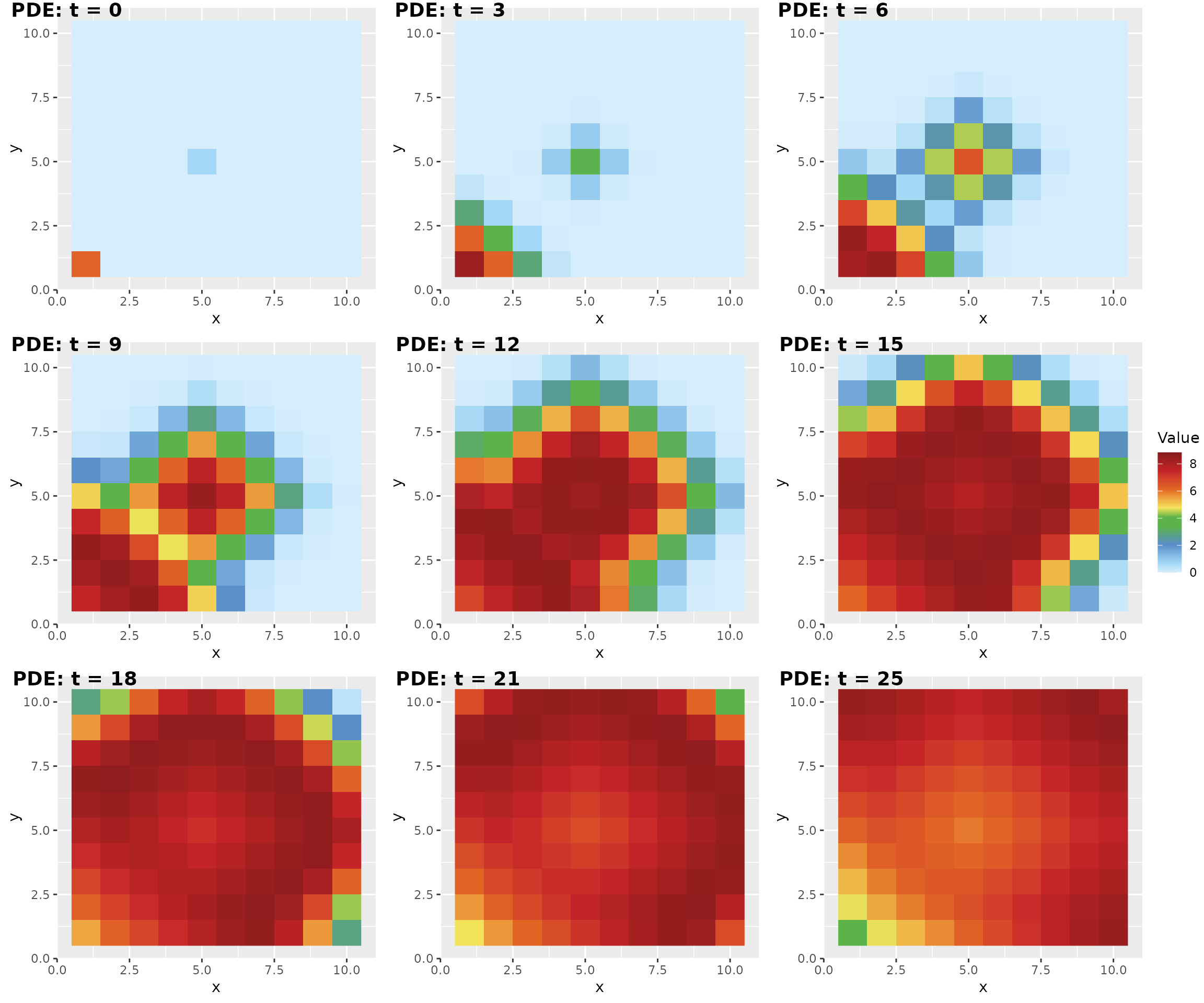
The heatmaps show how the spatial field changes over time under the true PDE simulator. This is the target pattern we want the emulator to reproduce.
5. Compare FFBS emulation with the PDE solution
Next, we compare the true PDE output with the FFBS emulator prediction. The top row shows the PDE simulator output, and the bottom row shows the exact posterior predictive mean from the emulator.
Good emulator performance should show similar spatial patterns in the two rows, especially at the main high- and low-value regions of the spatial field.
dat <- res_pre_exact
{
  plot_ls <- list()
  ind_sp <- data.frame(row = rep(1:Ny, times = Nx), col = rep(1:Nx, each = Ny))
  ind_plot <- 1

  for (i in tstamp) {
    temp <- dat[[i]][input_num,]
    rownames(temp) <- NULL
    colnames(temp) <- NULL
    dt <- data.frame(row = ind_sp$row, col = ind_sp$col, sol = temp)

    p <- ggplot(dt, aes(x = col, y = row, fill = sol)) +
      geom_raster() +
      scale_fill_gradientn(colours = col_bgr,
                           limits = c(0, max_y),
                           oob = scales::squish) +
      labs(x = "x", y = "y", fill = "Value")

    plot_ls[[ind_plot]] <- p
    ind_plot <- ind_plot + 1
  }
}

ffbs_heat <- plot_ls
labels <- c(
  paste0("PDE solution: t = ", tstamp[c(4, 6, 8)] - 1),
  paste0("FFBS emulation: t = ", tstamp[c(4, 6, 8)] - 1)
)

ggarrange(
  plotlist = list(
    pde_heat[[4]], pde_heat[[6]], pde_heat[[8]],
    ffbs_heat[[4]], ffbs_heat[[6]], ffbs_heat[[8]]
  ),
  ncol = 3,
  nrow = 2,
  labels = labels,
  font.label = list(size = 16, face = "bold"),
  hjust = -0.1,
  vjust = 1.2,
  align = "hv",
  common.legend = TRUE,
  legend = "right"
)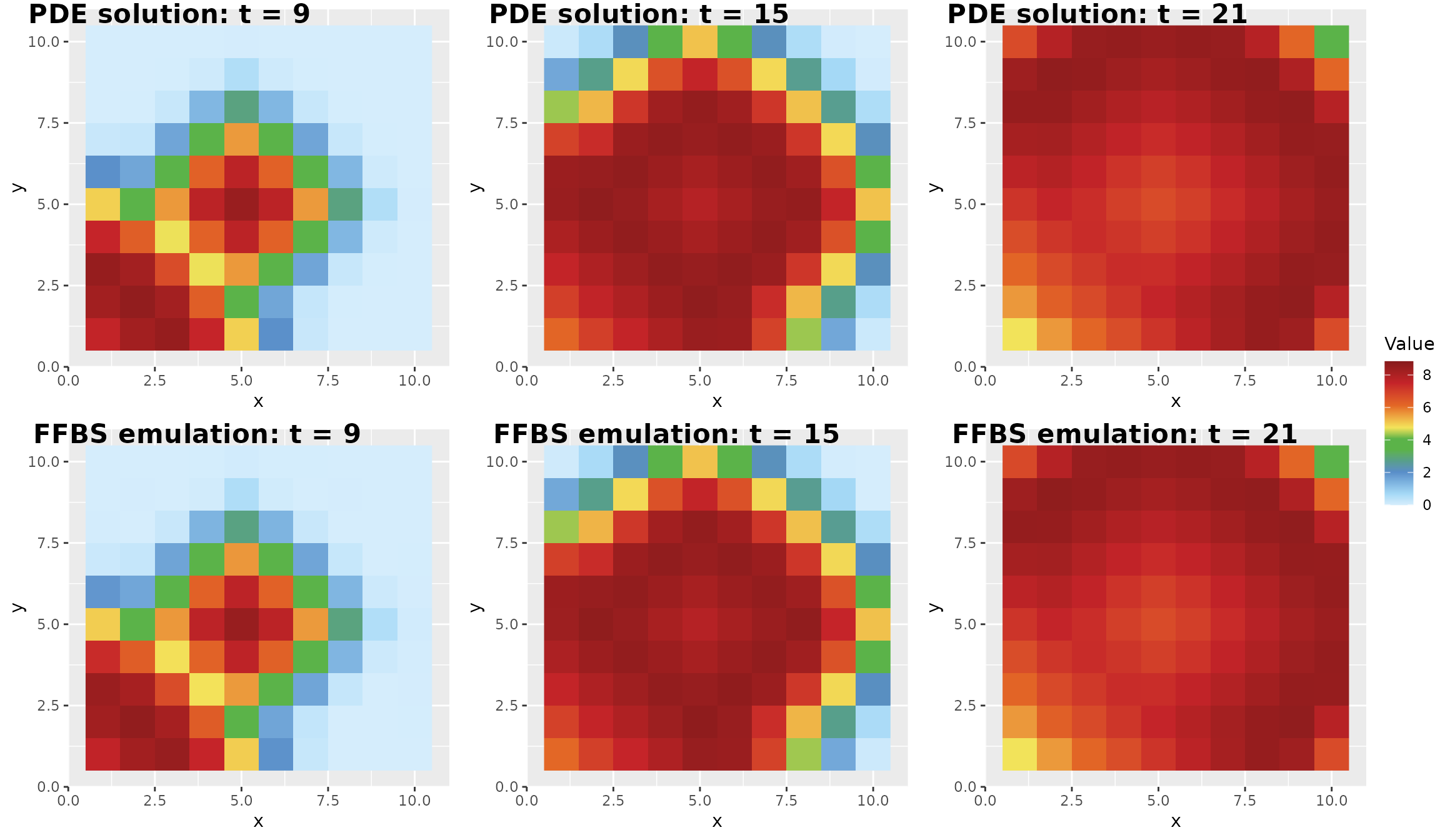
This side-by-side plot is a quick visual diagnostic. If the emulator misses important spatial features, possible next steps include increasing the number of training runs, changing the AR order, modifying the episode-window size, or tuning the GP covariance parameters.
6. Check predictive uncertainty
The MC output here consists of coefficient-conditioned mean samples. These intervals reflect coefficient uncertainty conditional on the supplied AR rows; they omit the conditional new-input GP field variance. The calibration vignette explicitly includes that covariance in its likelihood and field recovery. These conditional validation plots therefore do not by themselves establish full predictive coverage.
The Monte Carlo prediction res_pre_MC provides
coefficient-conditioned mean samples. We use those draws to compare the
predicted and true PDE values over all spatial locations for the
selected held-out input.
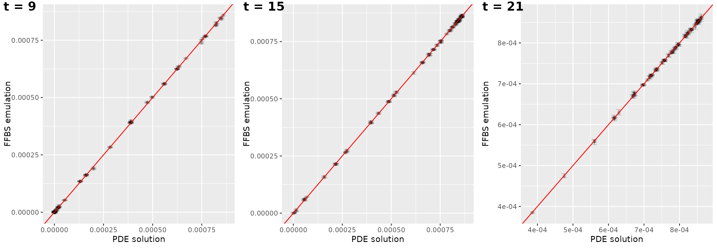
In each panel:
- the x-axis is the true PDE value,
- the y-axis is the posterior median of the FFBS prediction,
- vertical intervals show the 2.5th and 97.5th posterior predictive percentiles,
- the diagonal line represents perfect prediction.
Points close to the diagonal indicate accurate emulation. Wider intervals indicate larger predictive uncertainty.
{
  ### Error plot ----
  #### Specific time, one spatial location, all inputs ----
  {
    alpha_error <- 0.5
    res_pre <- res_pre_MC

    time_num <- 15
    sp_num <- 2
    y_true <- dt_pde_test[[time_num]][,sp_num]
    y_pre <- res_pre[[time_num]][,sp_num,]
    y_pre_stat <- data.frame(y_true = y_true,
                             med = apply(X = y_pre, MARGIN = 1, FUN = median),
                             lower = apply(X = y_pre, MARGIN = 1, FUN = quantile, prob = 0.025),
                             upper = apply(X = y_pre, MARGIN = 1, FUN = quantile, prob = 0.975))
    error_width <- (max(y_true) - min(y_true)) / 30 # denominator is for aesthetic
    ggplot(y_pre_stat, aes(x = y_true, y = med)) +
      geom_pointrange(aes(ymin = lower, ymax = upper), size =.2)+
      geom_errorbar(aes(ymin = lower, ymax = upper), width = error_width) +
      geom_abline(col = "red")
  }

  #### Specific time, one input, all spatial locations ----
  {
    time_num <- 20
    sp_num <- c(1:N_sp)
    y_true <- dt_pde_test[[time_num]][input_num,sp_num]
    y_pre <- res_pre[[time_num]][input_num,sp_num,]
    y_pre_stat <- data.frame(y_true = y_true,
                             med = apply(X = y_pre, MARGIN = 1, FUN = median),
                             lower = apply(X = y_pre, MARGIN = 1, FUN = quantile, prob = 0.025),
                             upper = apply(X = y_pre, MARGIN = 1, FUN = quantile, prob = 0.975))
    y_pre_stat <- y_pre_stat / N_people
    error_width <- (max(y_pre_stat["y_true"]) - min(y_pre_stat["y_true"])) / 30
    plot_error_1 <- ggplot(y_pre_stat, aes(x = y_true, y = med)) +
      geom_pointrange(aes(ymin = lower, ymax = upper), size =.2, alpha = alpha_error)+
      geom_errorbar(aes(ymin = lower, ymax = upper), width = error_width, alpha = alpha_error) +
      geom_abline(col = "red") +
      labs(x = "PDE solution", y = "FFBS prediction")
  }

  # panel
  time_p <- tstamp[c(4, 6, 8)]
  sp_num <- c(1:N_sp)
  plot_error_comp_ls <- list()
  plot_band_ls <- list()
  y_pre_stat_error_comp_ls <- list()
  for (t in 1:length(time_p)) {
    time_num <- time_p[t]
    y_true <- dt_pde_test[[time_num]][input_num,sp_num]
    y_pre <- res_pre[[time_num]][input_num,sp_num,]
    y_pre_stat <- data.frame(y_true = y_true,
                             med = apply(X = y_pre, MARGIN = 1, FUN = median),
                             lower = apply(X = y_pre, MARGIN = 1, FUN = quantile, prob = 0.025),
                             upper = apply(X = y_pre, MARGIN = 1, FUN = quantile, prob = 0.975))
    y_pre_stat <- y_pre_stat / N_people
    y_pre_stat_error_comp_ls[[t]] <- y_pre_stat
  }

  for (t in 1:length(time_p)) {
    # scatter plot
    error_width <- (max(y_pre_stat_error_comp_ls[[t]]["y_true"]) - min(y_pre_stat_error_comp_ls[[t]]["y_true"])) / 30
    plot_error_1 <- ggplot(y_pre_stat_error_comp_ls[[t]], aes(x = y_true, y = med)) +
      geom_pointrange(aes(ymin = lower, ymax = upper), size =.2, alpha = alpha_error / 3)+
      geom_errorbar(aes(ymin = lower, ymax = upper), width = error_width, alpha = alpha_error / 3) +
      geom_abline(col = "red") +
      labs(x = "PDE solution", y = "FFBS emulation")
    plot_error_comp_ls[[t]] <- plot_error_1

    # error band plot
    plot_band_predict <- ggplot(y_pre_stat_error_comp_ls[[t]], aes(x = y_true, y = med)) +
      geom_ribbon(aes(ymin = lower, ymax = upper, x = y_true), fill = "#A6CEE3", alpha = 1) +
      geom_point(aes(y = med), color = "#1F78B4", size = 0.7, alpha = 1) +
      geom_abline(color = "#E31A1C", linewidth = 1) +
      labs(x = "PDE solution", y = "FFBS emulation") +
      theme_minimal()
    plot_band_ls[[t]] <- plot_band_predict
  }
}
labels <- paste0("t = ", tstamp[c(4, 6, 8)] - 1)

ggarrange(
  plotlist = plot_error_comp_ls[1:3],
  ncol = 3,
  nrow = 1,
  labels = labels,
  font.label = list(size = 16, face = "bold"),
  hjust = -0.1,
  vjust = 1.2,
  align = "hv",
  common.legend = TRUE,
  legend = "right"
)
For a package vignette, we use a small value of nsam so
that the example runs quickly. In real applications, you should increase
nsam if you want more stable posterior uncertainty
summaries.
Practical tips
- Start with
AR_choice = 1orAR_choice = 2. AR(2) can capture richer temporal dependence but creates a larger state vector. - Increase
episode_windowonly when you want each block to contain a wider spatial strip. Larger blocks may capture more spatial structure but require more computation. - Tune
gp_tune,gp_sigma2, andgp_tau2when predictions appear too smooth, too noisy, or poorly calibrated. - Use exact prediction for fast point prediction and MC prediction when uncertainty intervals are needed.
- Keep the training and prediction inputs on the same scale before constructing the GP covariance.
Summary
This tutorial showed how to use spDBL to build an FFBS
emulator for time-indexed spatial PDE outputs. The workflow has four
main steps:
- Load the training and test PDE data.
- Fit the emulator with
emulator_learn(). - Predict held-out PDE outputs with
emulator_predict(). - Evaluate the emulator using heatmaps and uncertainty plots.
The wrapper functions in this vignette are intended to be reusable starting points. For a new PDE simulator, the main changes are usually the data-loading step, the spatial grid dimensions, the AR order, and the GP covariance tuning parameters.